38 change data labels in excel chart

Format Data Labels in Excel- Instructions - TeachUcomp, Inc. Nov 14, 2019 — To format data labels in Excel, choose the set of data labels to format. To do this, click the “Format” tab within the “Chart Tools” contextual ... Move data labels - support.microsoft.com Click any data label once to select all of them, or double-click a specific data label you want to move. Right-click the selection > Chart Elements > Data Labels arrow, and select the placement option you want. Different options are available for different chart types.

Add or remove data labels in a chart - support.microsoft.com Click the data series or chart. To label one data point, after clicking the series, click that data point. In the upper right corner, next to the chart, click Add Chart Element > Data Labels. To change the location, click the arrow, and choose an option. If you want to show your data label inside a text bubble shape, click Data Callout.

Change data labels in excel chart

Excel charts: add title, customize chart axis, legend and data labels ... Adding data labels to Excel charts. To make your Excel graph easier to understand, you can add data labels to display details about the data series. ... Data label tips: To change the position of a given data label, click it and drag to where you want using the mouse. To change the labels' font and background color, select them, ... How to Add Axis Label to Chart in Excel - Sheetaki Method 1: By Using the Chart Toolbar. Select the chart that you want to add an axis label. Next, head over to the Chart tab. Click on the Axis Titles. Navigate through Primary Horizontal Axis Title > Title Below Axis. An Edit Title dialog box will appear. In this case, we will input "Month" as the horizontal axis label. Next, click OK. You ... How to add data labels from different column in an Excel chart? Right click the data series in the chart, and select Add Data Labels > Add Data Labels from the context menu to add data labels. 2. Click any data label to select all data labels, and then click the specified data label to select it only in the chart. 3.

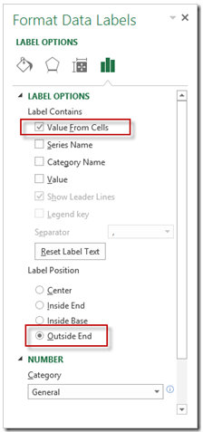
Change data labels in excel chart. Change the format of data labels in a chart To get there, after adding your data labels, select the data label to format, and then click Chart Elements > Data Labels > More Options. To go to the appropriate area, click one of the four icons ( Fill & Line, Effects, Size & Properties ( Layout & Properties in Outlook or Word), or Label Options) shown here. How to create Custom Data Labels in Excel Charts Right click on any data label and choose the callout shape from Change Data Label Shapes option. Now adjust each data label as required to avoid overlap. Put solid fill color in the labels Finally, click on the chart (to deselect the currently selected label) and then click on a data label again (to select all data labels). Custom Data Labels with Colors and Symbols in Excel Charts - [How To] To apply custom format on data labels inside charts via custom number formatting, the data labels must be based on values. You have several options like series name, value from cells, category name. But it has to be values otherwise colors won't appear. Symbols issue is quite beyond me. How to Use Cell Values for Excel Chart Labels Select the chart, choose the "Chart Elements" option, click the "Data Labels" arrow, and then "More Options." Uncheck the "Value" box and check the "Value From Cells" box. Select cells C2:C6 to use for the data label range and then click the "OK" button. The values from these cells are now used for the chart data labels.

2/ Right-click i.e. on the 1st histo. bar (A) > Add Data Labels (numbers are displayed a the top of the bars) 3/ Click one of the numbers that just displayed (the Format Data Labels pane opens on the right) > Check option "Value From Cells" > Select range C2:C7 > OK > Uncheck option "Value" demo.png (18.5 KiB) · 3 Excel Chart Data Labels-Modifying Orientation - Microsoft Community Replied on September 14, 2016 In reply to PaulaAB's post on September 13, 2016 Hi Paula, You can right click on the data label part then select Format Axis. Click on the Size & Properties tab then adjust the Text Direction or Custom Angle. Thanks, Mike Report abuse 6 people found this reply helpful · Was this reply helpful? Replies (7) Create Dynamic Chart Data Labels with Slicers - Excel Campus Step 6: Setup the Pivot Table and Slicer. The final step is to make the data labels interactive. We do this with a pivot table and slicer. The source data for the pivot table is the Table on the left side in the image below. This table contains the three options for the different data labels. How to add or move data labels in Excel chart? In Excel 2013 or 2016. 1. Click the chart to show the Chart Elements button . 2. Then click the Chart Elements, and check Data Labels, then you can click the arrow to choose an option about the data labels in the sub menu. See screenshot: In Excel 2010 or 2007. 1. click on the chart to show the Layout tab in the Chart Tools group. See ...

Edit titles or data labels in a chart - support.microsoft.com The first click selects the data labels for the whole data series, and the second click selects the individual data label. Right-click the data label, and then click Format Data Label or Format Data Labels. Click Label Options if it's not selected, and then select the Reset Label Text check box. Top of Page How to Rename a Data Series in Microsoft Excel To do this, right-click your graph or chart and click the "Select Data" option. This will open the "Select Data Source" options window. Your multiple data series will be listed under the "Legend Entries (Series)" column. To begin renaming your data series, select one from the list and then click the "Edit" button. How to format axis labels as thousands/millions in Excel? Reuse Anything: Add the most used or complex formulas, charts and anything else to your favorites, and quickly reuse them in the future. More than 20 text features: Extract Number from Text String; Extract or Remove Part of Texts; Convert Numbers and Currencies to English Words. Merge Tools: Multiple Workbooks and Sheets into One; Merge Multiple Cells/Rows/Columns Without Losing Data; Merge ... How to Customize Your Excel Pivot Chart Data Labels - dummies To add data labels, just select the command that corresponds to the location you want. To remove the labels, select the None command. If you want to specify what Excel should use for the data label, choose the More Data Labels Options command from the Data Labels menu. Excel displays the Format Data Labels pane.

Microsoft Excel Tutorials: The Chart Layout Panels

How to rotate axis labels in chart in Excel? Go to the chart and right click its axis labels you will rotate, and select the Format Axis from the context menu. 2. In the Format Axis pane in the right, click the Size & Properties button, click the Text direction box, and specify one direction from the drop down list. See screen shot below: The Best Office Productivity Tools

How to Add Data Labels to an Excel 2010 Chart - dummies

Change axis labels in a chart - support.microsoft.com Right-click the category labels you want to change, and click Select Data. In the Horizontal (Category) Axis Labels box, click Edit. In the Axis label range box, enter the labels you want to use, separated by commas. For example, type Quarter 1,Quarter 2,Quarter 3,Quarter 4. Change the format of text and numbers in labels

How-to Use Data Labels from a Range in an Excel Chart - Excel Dashboard Templates

excel - Change format of all data labels of a single series at once ... Workaround 1: Fill up all empty cells referred to. Change the format of labels. Remove added contents. Workaround 2: Change to a dummy range for the data labels, which has no empty cells. Change the format of labels. Switch back to your intended range.

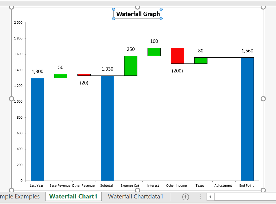
Waterfall Chart Templates (Excel 2010 and 2013) – Edward Bodmer – Project and Corporate Finance

How to change chart axis labels' font color and size in Excel? Right click the axis you will change labels when they are greater or less than a given value, and select the Format Axis from right-clicking menu. 2. Do one of below processes based on your Microsoft Excel version:

create excel spreadsheet for your data for $5 - SEOClerks

Add / Move Data Labels in Charts - Excel & Google Sheets Adding Data Labels Click on the graph Select + Sign in the top right of the graph Check Data Labels Change Position of Data Labels Click on the arrow next to Data Labels to change the position of where the labels are in relation to the bar chart Final Graph with Data Labels

Excel Course: Inserting Graphs

Custom Chart Data Labels In Excel With Formulas Follow the steps below to create the custom data labels. Select the chart label you want to change. In the formula-bar hit = (equals), select the cell reference containing your chart label's data. In this case, the first label is in cell E2. Finally, repeat for all your chart laebls.

Share :