45 how to add data labels to a 3d pie chart in excel
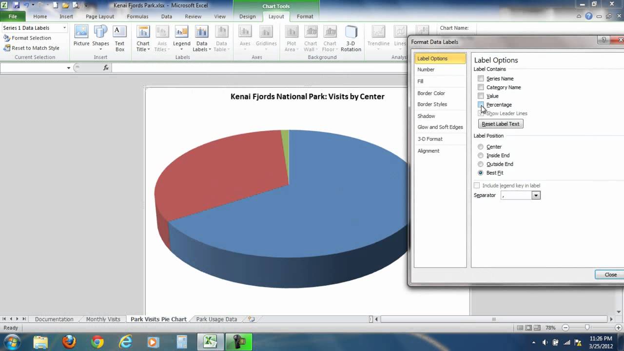
How to Create and Format a Pie Chart in Excel - Lifewire 23 Jan 2021 — Add Data Labels to the Pie Chart · Select the plot area of the pie chart. · Right-click the chart. Screenshot of right-click menu · Select Add Data ... PIE CHART in R with pie() function [WITH SEVERAL EXAMPLES] An alternative to display percentages on the pie chart is to use the PieChart function of the lessR package, that shows the percentages in the middle of the slices.However, the input of this function has to be a categorical variable (or numeric, if each different value represents a category, as in the example) of a data frame, instead of a numeric vector.
How to create graphs in Illustrator - Adobe Inc. 23.5.2022 · Enter labels for the different sets of data in the top row of cells. These labels will appear in the legend. If you don’t want Illustrator to generate a legend, don’t enter data‑set labels. Enter labels for the categories in the left column of cells. Categories are often units of time, such as days, months, or years.
How to add data labels to a 3d pie chart in excel
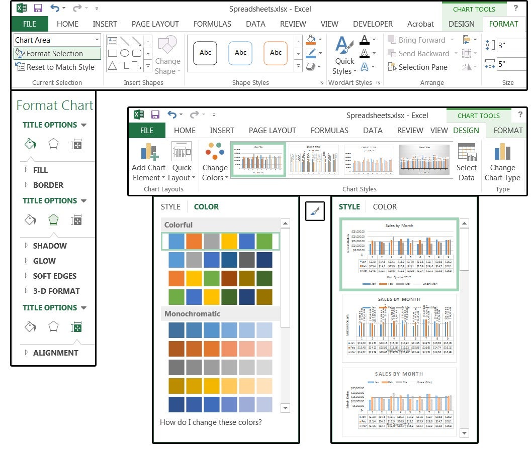
How to Label a Pie Chart in Excel (6 Steps) - ItStillWorks Clicking on the data series or a specific data point will open the "Chart Tools" tab. Locate the "Labels" group and click on the "Layout" tab. Click the "Data ... How To Add and Remove Legends In Excel Chart? - EDUCBA This has been a guide to Legend in Chart. Here we discuss how to add, remove and change the position of legends in an Excel chart, along with practical examples and a downloadable excel template. You can also go through our other suggested articles – Line Chart in Excel; Excel Bar Chart; Pie Chart in Excel; Scatter Chart in Excel how to create a shaded range in excel — storytelling with data 8.10.2019 · Adding a shaded region to depict a range of values in Excel - a how-to for making better data visualizations. ... Add a new data series for the Minimum by right-clicking the chart and choosing “Select Data”: ... one 3D pie at a time!
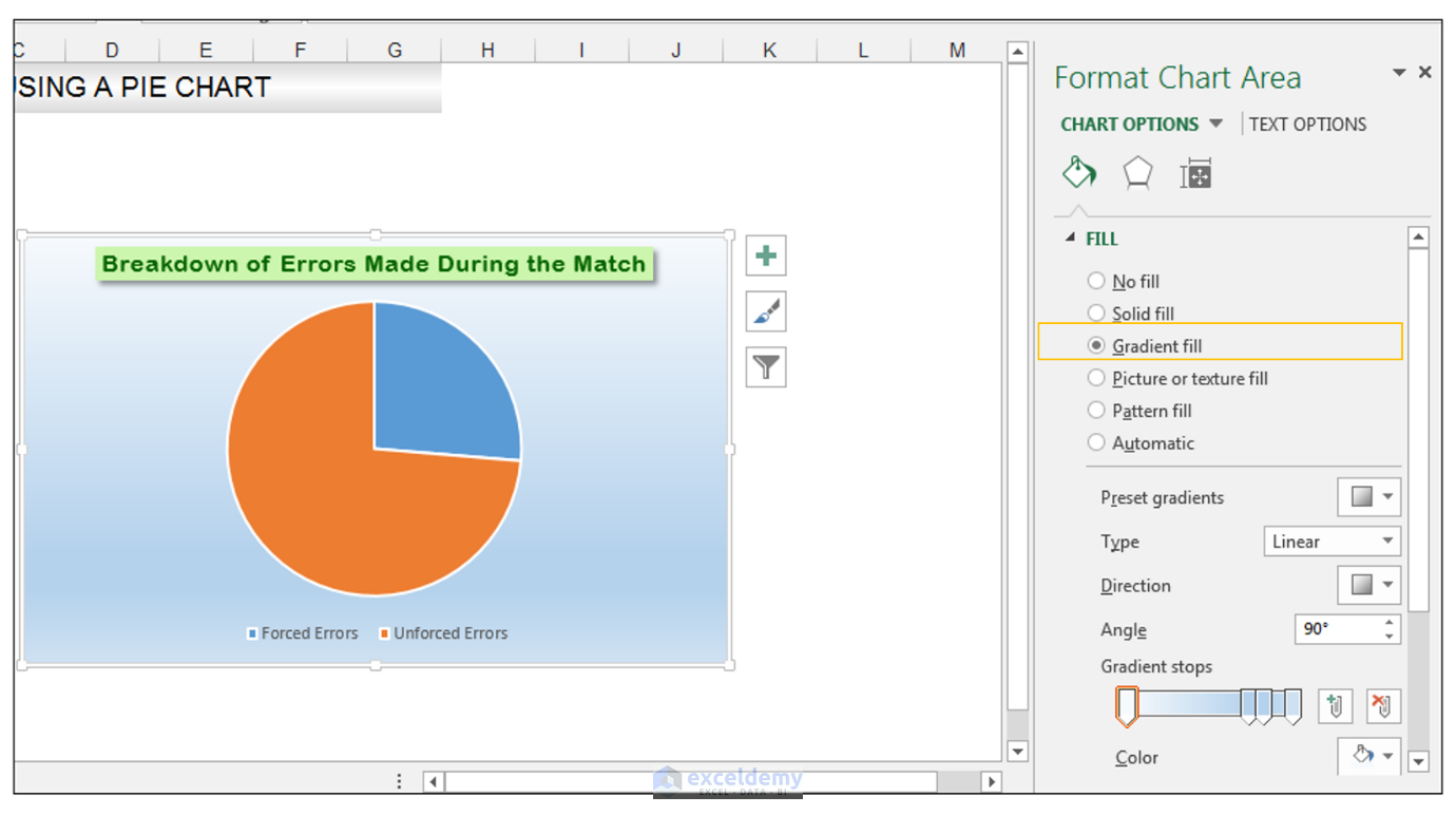
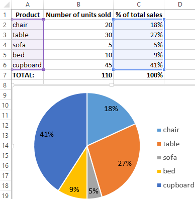
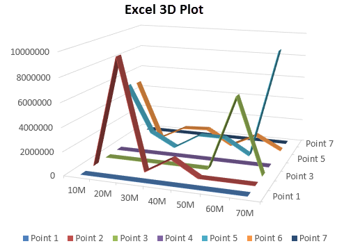
How to add data labels to a 3d pie chart in excel. Excel 3-D Pie charts 1. Select the data range (in this example, B5:C10). · 2. On the Insert tab, in the Charts group, choose the Pie button: · 3. Right-click in the chart area, then ... How to Show Percentages in Stacked Column Chart in Excel? 17.12.2021 · Step 4: Add Data labels to the chart. Goto “Chart Design” >> “Add Chart Element” >> “Data Labels” >> “Center”. You can see all your chart data are in Columns stacked bar. Step 5: Steps to add percentages/custom values in Chart. Create a percentage table for your chart data. Copy header text in cells “b1 to E1” to cells “G1 ... How to Make a Scatter Plot in Excel (XY Chart) - Trump Excel While you can use third-party add-ins and tools to do this, I cannot think of any additional benefit that you will get with a 3D scatter chart as compared to a regular 2D scatter chart. In fact, I recommend staying away from any kind of 3D chart as it has the potential of misrepresenting the data and portions in the chart. 3D Plot in Excel | How to Plot 3D Graphs in Excel? - EDUCBA Do not add data labels in 3D Graphs because the plot gets congested many time. Use data labels when it is actually visible. Recommended Articles. This has been a guide to 3D Plot in Excel. Here we discussed How to plot 3D Graphs in Excel along with practical examples and a downloadable excel template.
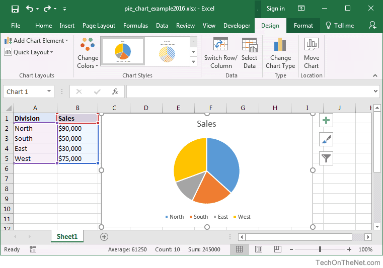
Tips for turning your Excel data into PowerPoint charts 21.8.2012 · 3. When you click OK, a temporary Excel spreadsheet opens, with dummy data. This spreadsheet is named “Chart in Microsoft PowerPoint.” Now navigate to your Excel spreadsheet that contains the data you want for your chart, select the data, and copy it to the clipboard. 4. Go back to the temporary spreadsheet, click in cell A1, and paste. 5. Free Pie Chart Maker - Make Your Own Pie Chart | Visme To use the pie chart maker, click on the data icon in the menu on the left. Enter the Graph Engine by clicking the icon of two charts. Choose the pie chart option and add your data to the pie chart creator, either by hand or by importing an Excel or Google sheet. How to Create a Pie Chart in Google Sheets - Lido How to create a 3D pie chart. Another type of pie chart that you can create in Google Sheets is the 3D pie chart. Just like pie chart and doughnut chart, the choice of using a 3D pie chart depends on the aesthetics. Note, however, that the use of 3D pie charts is discouraged because it causes misinterpretations regarding the data visualized. how to create a shaded range in excel — storytelling with data 8.10.2019 · Adding a shaded region to depict a range of values in Excel - a how-to for making better data visualizations. ... Add a new data series for the Minimum by right-clicking the chart and choosing “Select Data”: ... one 3D pie at a time!
How To Add and Remove Legends In Excel Chart? - EDUCBA This has been a guide to Legend in Chart. Here we discuss how to add, remove and change the position of legends in an Excel chart, along with practical examples and a downloadable excel template. You can also go through our other suggested articles – Line Chart in Excel; Excel Bar Chart; Pie Chart in Excel; Scatter Chart in Excel How to Label a Pie Chart in Excel (6 Steps) - ItStillWorks Clicking on the data series or a specific data point will open the "Chart Tools" tab. Locate the "Labels" group and click on the "Layout" tab. Click the "Data ...
How to Create Excel Pie Charts & Add Rich Data Labels to The Chart!
Creating a 3D Pie Chart in Excel Vid.wmv - YouTube

Creating Pie Chart and Adding/Formatting Data Labels (E... | Doovi
Excel charts: Mastering pie charts, bar charts and more | PCWorld
MS Office Suit Expert : MS Excel 2016: How to Create a Pie Chart
Add and take the percent from number in Excel with the examples

How to Create a Pie Chart in Excel | Smartsheet
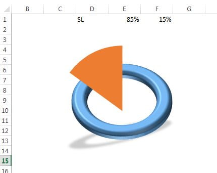
3D Doughnut Chart for KPI Metrics - PK: An Excel Expert

How to Make a Pie Chart in Microsoft Excel 2010
3D Plot in Excel | How to Plot 3D Graphs in Excel?

How to Make a Pie Chart in Excel & Add Rich Data Labels to The Chart!

33 How To Label A Pie Chart In Excel - Labels 2021
:max_bytes(150000):strip_icc()/Capture-5c84941446e0fb00013364fc.JPG)
How to Create and Format a Pie Chart in Excel
How to Create Excel Pie Charts & Add Rich Data Labels to The Chart!

How to Make a Pie Chart in Excel & Add Rich Data Labels to The Chart!
Inserting % and Actual Value in Labels for Pie Chart

74 MICROSOFT EXCEL HOW TO CREATE 2D PIE CHART - YouTube
Create a Pie Chart in Excel - Easy Excel Tutorial
Post a Comment for "45 how to add data labels to a 3d pie chart in excel"