38 how to add data labels in excel bar chart

Stocks Earnings Calendar & Dividends Calendar - Barchart.com Barchart Premier Barchart for Excel No-Ads Barchart Free Membership Watchlist Portfolio Portfolio Summary Alert Center Alert Templates Screener My Charts Custom Views Chart Templates Compare Stocks Daily Prices Download Historical Data Download ... As with all data tables on the site, you can re-sort the table by clicking on any column heading ... How to Label a Series of Points on a Plot in MATLAB You can label points on a plot with simple programming to enhance the plot visualization created in MATLAB ®. You can also use numerical or text strings to label your points. Using MATLAB, you can define a string of labels, create a plot and customize it, and program the labels to appear on the plot at their associated point. MATLAB Video Blog

Tableau Desktop vs Microsoft Excel Excel allows you to plot the results of your analysis but Tableau actually helps perform better analysis. The entire process is visual so you get the benefits of the clean, simple presentation of a chart at every step along the way. This encourages data exploration and allows people to understand the data instead of just presenting a report.

How to add data labels in excel bar chart

Developer - Microsoft Power BI Community Custom visual creation, API usage, real-time dashboards, integrating with Power BI, content packs. Basically, everything about extending Power BI. Descriptive data analysis: COUNT, SUM, AVERAGE, and other calculations 1. In the formula bar, type: = click in the cell containing the count of males. this cell reference (e.g., C27) should now be written in the formula bar after the equals sign (=) 3. click back into the formula bar and type: / 4. click in the cell containing the total count of students. 5. click back into the formula bar and finish the bracket:) How to add filter to column in excel (Step-by-Step) | WPS Office Academy 1. To filter a column, click the drop-down arrow next to it. 2. To easily deselect all data, uncheck the Select All box. 3. Click OK after checking the boxes next to the data you wish to see. This is how, for example, we may filter data in the Region column to see just sales from the East and North: 4. Done!

How to add data labels in excel bar chart. Junk Charts The left column shows the original charts from the article. In both charts, the two cars are so close together that it is impossible to learn the scale of the difference. The amount of difference is a fraction of the width of a car icon. The right column shows the "self-sufficiency test". Imagine the data labels are not on the chart. How to Customize Histograms in MATLAB - Video - MathWorks Finally, to give us more control on how our histogram is visualized, we'll convert the histogram into a bar graph. We simply replace "histogram" with "histcounts" to get the count in each bin, and the bin edges. Note that we only need to supply the "count" variable to the bar function to reproduce the shape of the histogram. Customizing Graphs and Charts - NI Right-click the graph or chart and select Visible Items»Graph Palette from the shortcut menu to display the graph palette, shown as follows. Click a button in the graph palette to move cursors, zoom, or pan the display. Each button displays a green LED when you enable the button. Library Guides: IEEE Referencing: Figures, tables and equations Figures, tables and equations from another source. Figures are visual presentations of results, such as graphs, diagrams, images, drawings, schematics, maps, etc. If you are referring to a specific figure, table or equation found in another source, place a citation number in brackets directly after its mention in the text, and then use the ...

116+ Microsoft Access Databases And Templates With Free Examples ... 4. Data that is processed using an access (database) table can produce more than one display model, each of which has its own functions. Both models (tables and reports) of this data sheet can be printed as well. While in Excel, it will depend on the type of table that is processed and arranged only. 5. Both Excel and Access can display sort data. Zach, Author at Statology How to Print Pandas DataFrame with No Index. July 21, 2022 by Zach. You can use the following methods to print a pandas DataFrame without the index: Method 1: Use to_string () Function print (df.to_string (index=False)) Method 2: Create Blank Index…. Uncategorized. Grouping Data - SPSS Tutorials - LibGuides at Kent State University Click Data > Split File. Select the option Compare groups. Double-click the variable Gender to move it to the Groups Based on field. When you are finished, click OK. After splitting the file, the only change you will see in the Data View is that data will be sorted in ascending order by the grouping variable (s) you selected. Creating Reports and Graphs - Quicken Go to the Reports dropdown in the top menu bar. You will find various standard reports. You can select one of these or you can go to Reports & Graphs Center. In the Quicken Standard Reports list on the left, click the section you want. Select the report or graph you want. Quicken displays the settings you can adjust before you create the report.

[Solved] : How to Fix MS Excel Crash Issue - Article Restart Excel in normal mode and go to File> Options> Add-ins Choose COM Add-ins from the drop-down and click Go Uncheck all the checkboxes and click OK Restart Excel and check if the issue is resolved If Excel doesn't crash or freeze anymore, open COM Add-ins and enable one add-in at a time followed by Excel restart. My Charts - Barchart.com The "My Charts" feature, available to Barchart Premier Members, lets you build a portfolio of personalized charts that you can view on demand. Save numerous chart configurations for the same symbol, each with their own trendlines and studies. Save multiple commodity spread charts and expressions, view quote and technical analysis data, and more. How to Add the Last Refreshed Date and Time to a Power BI Report Now click on the Advanced Editor option, from the Home ribbon, and paste the M code (see below). let. Source = #table (type table [Date Last Refreshed=datetime], { {DateTime.LocalNow ()}}) in. Source. The M code creates a column with the name Date Last Refreshed and it gathers the current date and time. The Advanced Editor window for Date Last ... SPSS Tutorials: Frequency Tables - Kent State University To request the mode statistic, click Statistics. Check the box next to Mode, then click Continue. To turn on the bar chart option, click Charts. Select the radio button for Bar Charts. Then click Continue. When finished, click OK. Using Syntax FREQUENCIES VARIABLES=Rank /STATISTICS=MODE /BARCHART FREQ /ORDER=ANALYSIS. Output

storytelling with data: May 2013

Microsoft Excel Basics - Research Guides at MCPHS University = (B2+C2+D2)/3 Adds contents of B2, C2, and D2 and divides result by 3 Excel also has built-in functions that can do a lot of useful calculations. These are most easily accessed by hitting the Insert Function button, which is represented by the "fx" symbol next to the formula bar.

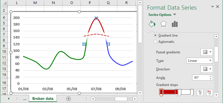
Creating a chart with critical zones

How to Build Basic Reports (Horizon Analytics) - Gainsight Inc. Select Object and Fields. To select Object and Fields: From the Select Object dropdown list, select the Data Source. Here, Matrix Data source is selected, and once selected the data source will display all the Gainsight objects. Select or search the required object. All the fields from the selected object will be displayed in the Fields section.; Enter the field name in the Fields Search bar ...

30 Label The Excel Window - Labels Design Ideas 2020

Figures (graphs and images) - APA 7th Referencing Style Guide - Library ... The first option is to place all figures on separate pages after the reference list. The second option is to embed each figure within the text.

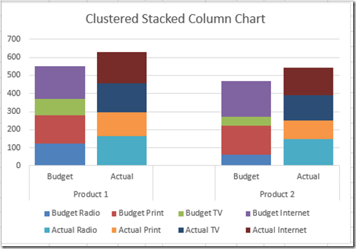
How-to Make an Excel Clustered Stacked Column Chart with Different Colors by Stack - Excel ...

How to Create a Power BI Date Range Slicer - Ask Garth Drag the date column (#3) from the dataset (in my case it's WIR checkdate) and place it in the Field section (#4) of the slicer. The slicer automatically picks up the start date and the end date from the date column and adds the column name to the slicer heading as a title (#5). In this case it's, "Date_Checked."

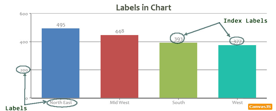
Tutorial on Labels & Index Labels in Chart | CanvasJS JavaScript Charts

microsoft excel - Bar chart reduce number of labels by creating Others ... 1. Suppose you have a pivot table like this: Put your cursor in the values column (column E in the picture above). Then right click, Sort, Sort smallest to largest. Like this: Now in the column that says "Row Labels", select the fruits you want to group as others. Then right-click and select 'Group'. Like this:

How to Create A Brain-Friendly Stacked Bar Chart in Excel

Contextures Excel Resources to Help You Succeed Many More Excel Tutorials. Next, you can check out these popular Excel tutorials.. 1 -- Key Skills in Excel - Do you know all of these key Excel skills? 2 -- How to Count Specific Cells - Count items in a list, based on one or more criteria 3 -- How to Do a VLOOKUP - Find a lookup item in a table, such price for a specific product 4 -- Create a Pivot Table - Summarize thousands of rows of data ...

How To Make Awesome Ranking Charts With Excel Pivot Tables - Moz

Tips and tricks for formatting in reports - Power BI Now imagine you want to call out the Extreme segment to show how well this brand new segment is performing, by using color. Here are the steps: Expand the Data colors card and turn the slider On for Show all. This displays the colors for each data element in the visualization. You can now modify any of the data points. Set Extreme to orange.

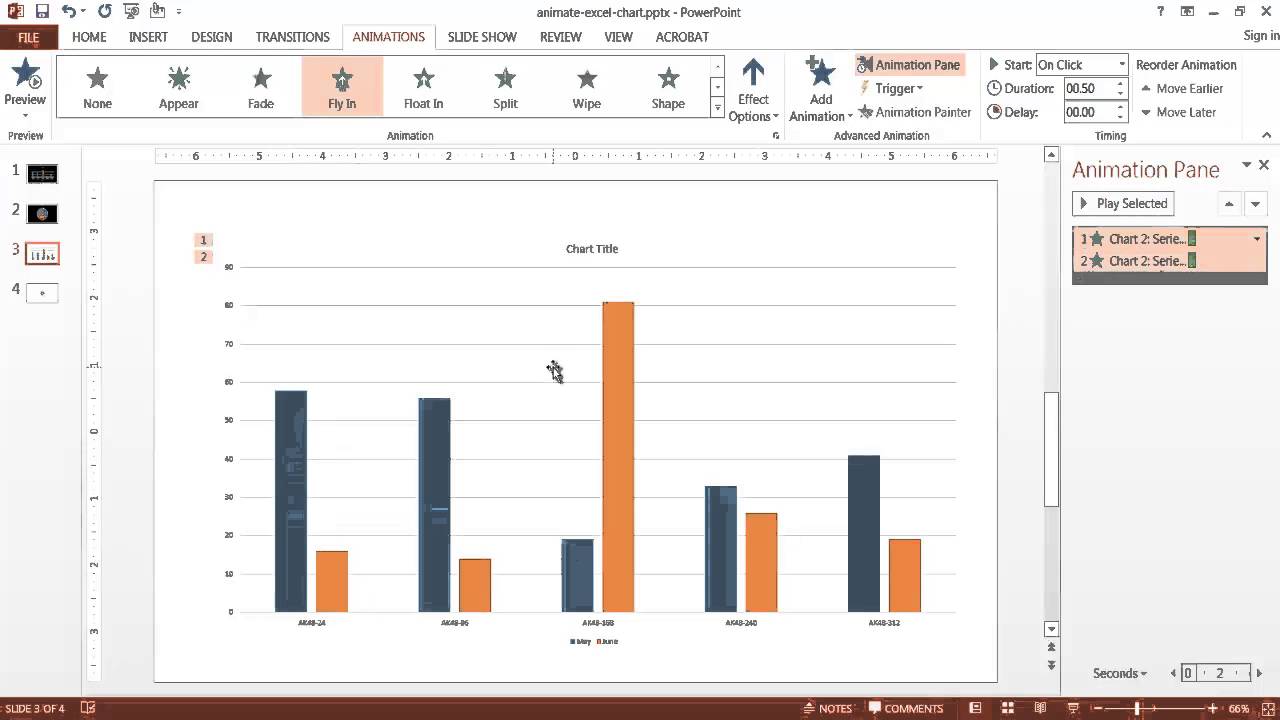
Animate an Excel Chart in PowerPoint - YouTube

The Global Temperature Record Says We're in a "Climate Emergency", It's ... Always Look at the Axes on a Chart. Adjusting the axes of a graph to make a point is a classic technique in manipulating charts. As a first principle, the y-axis on a bar chart should always start at 0. If not, it's easy to prove an argument by manipulating the range, by, for example, turning minor increases into massive changes:

Share :